Linear Regression in Machine Learning with Python & Sklearn

Linear regression is a fundamental machine learning algorithm used extensively across various industries, from finance and healthcare to marketing and sports analytics.

This tutorial will teach you how to implement linear regression using Python and Scikit-Learn (Sklearn), a popular open-source library for data science in Python.

By the end of this, you’ll have a solid understanding of what linear regression is, why it’s important, how to prepare your data for training linear regression models, and how to use Sklearn to build and evaluate linear regression models. Let’s get started!

Linear regression is a supervised machine learning algorithm that allows us to model the relationship between one or more independent variables (also known as predictors) and a dependent variable, which we want to predict.

The goal of linear regression is to find the best-fit line or plane that describes this relationship in our data. For example, in simple linear regression, where there’s only one independent variable (x), the equation is:

where y represents the dependent variable (what we’re trying to predict), x represents the independent variable, m is the slope of the line, and b is the intercept. In multiple linear regression, which involves more than one independent variable, the equation becomes:

where y remains our dependent variable, x1 through Xn are our independent variables, and w1 through wn are their respective weights or coefficients.

The goal of linear regression is to find the best values for these weights (w) and intercept (b) that minimize the error (the difference) between our predicted values and the actual observed values in our dataset.

Linear regression can be applied across various domains due to its simplicity, interpretability, and versatility. It also serves as a foundation for other advanced machine learning techniques like logistic regression, decision trees, random forests, support vector machines, and neural networks.

The most common libraries used in data science are:

1. Pandas: Pandas is used for data manipulation, handling missing values, and creating data frames. It provides fast, flexible, and expressive data structures with strong handling of real-world data and a wide range of built-in data analysis functions.
2. NumPy: NumPy is the fundamental package for scientific computing in Python. It provides support for large multi-dimensional arrays and matrices, along with a collection of high-level mathematical functions to operate on these arrays.
3. Matplotlib: Matplotlib is a plotting library that allows you to visualize your data.
4. Scikit-Learn (Sklearn): Sklearn provides easy-to-use tools for machine learning in Python, including linear regression models and other supervised and unsupervised learning algorithms.

We will be using the California Housing Dataset, a popular dataset that can be accessed from Scikit-Learn, to demonstrate linear regression. It is a dataset containing information about housing information in California, including features like median income and average number of rooms. Our goal will be to predict the median house value based on these features using simple linear regression.

Let’s start by importing the necessary libraries:

# Import the necessary libraries
import numpy as np
import pandas as pd
# Sklearn datasets library provides a few toy datasets to work with, one of which is the California housing dataset
from sklearn.datasets import fetch_california_housing
# Import the Linear Regression model from sklearn
from sklearn.linear_model import LinearRegression
# Import the train_test_split function from the model_selection module
from sklearn.model_selection import train_test_split
# Import the mean_squared_error, mean_absolute_error, and r2_score functions from the metrics module
from sklearn.metrics import mean_squared_error, mean_absolute_error, r2_score
# Import Matplotlib and Seaborn
import matplotlib.pyplot as plt
import seaborn as sns

Next, let’s load our dataset:

# Load the California Housing data set
data = fetch_california_housing()
# Display some information about the dataset
print(data.DESCR)

Here are the features of the california housing dataset:

1. MedInc: median income (dollars) in a block group
2. HouseAge: median house age in years within a block group
3. AveRooms: average number of rooms per household in a block group
4. AveBedrms: average number of bedrooms per household in a block group
5. Population: total population for the entire block group
6. AveOccup: average number of household members within a block group
7. Latitude: latitudinal coordinate of the block group’s centroid
8. Longitude: longitudinal coordinate of the block group’s centroid

# Create a pandas DataFrame from the data
df = pd.DataFrame(data.data, columns=data.feature_names)
# Add the target variable to the DataFrame
df['target'] = data.target

Here is how the data looks like:

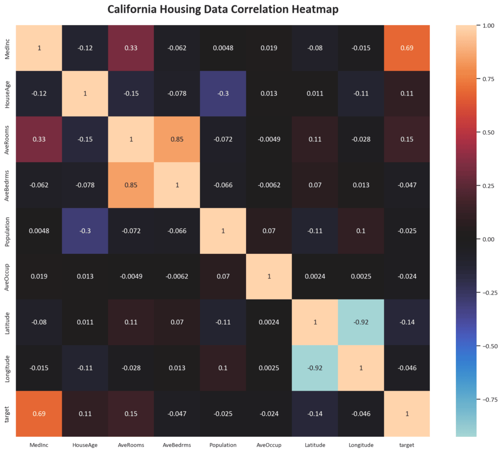
We will choose a feature we can use for simple linear regression then compare the performance with multiple linear regression. Let’s plot the correlation between the features and the target variable to choose the feature we can use for simple linear regression.

We will use seaborn, a popular data visualization library based on matplotlib, to plot the correlation matrix.

import matplotlib.pyplot as plt
import seaborn as sns
# Plot the correlation between the features and the target variable
plt.figure(figsize=(20, 16))
sns.heatmap(df.corr(), annot=True, cmap='mako', center=0)
plt.title('California Housing Data Correlation Heatmap', fontsize=20, fontweight='bold', pad=20, fontname='Arial')
plt.xticks(fontsize=12)

As we can see, the feature MedInc has the highest correlation with the target variable, followed by AveRooms. We will use MedInc for simple linear regression and then use all the features for multiple linear regression.

Next, let’s split the data into training and test sets. This is standard practice in machine learning to evaluate the performance of the model.

We train the model on the training set and evaluate it on the test set. This helps us to estimate how well the model will generalize, or capture the underlying patterns, which allows it to make accurate predictions on new, unseen data.

We will use the train_test_split function from Scikit-Learn:

# Split into training and testing sets with a ratio of 80% to 20%
X_train, X_test, y_train, y_test = train_test_split(df['MedInc'].values, df['target'].values, test_size=0.2, random_state=0)

Here, the train_test_split function splits the data into training and test sets, the first two parameters are the input data and target, which are X and y, respectively.

The test_size parameter specifies the ratio of the test set, which is set to 0.2, meaning that 20% of the data will be used for testing and the remaining 80% for training. The random_state parameter sets a seed for the random number generator, which allows us to reproduce the results.

Next, let’s train the linear regression model on the training data. We will use the fit method of the linear regression object and pass the training data as arguments:

# Create a Linear Regression model
simple_model = LinearRegression()
# Fit the model on the training data
simple_model.fit(X_train, y_train)
# Make predictions on the testing data
simple_predictions = simple_model.predict(X_test)

In this step, the linear regression model is trained on the training data. When we say “training” a machine learning model, it means teaching or feeding the algorithm with data so it can learn to make predictions on new, unseen data.

In this case, our Linear Regression model is trying to find the best-fit line (the coefficients for the equation y = mx + b) that minimizes the sum of squared errors between the actual and predicted values in our training dataset.

The goal here is to minimize the residual sum of squares (RSS), which is the sum of the squared differences between the observed target variable y_train and the predicted target variable ŷ. The model will adjust its coefficients until it finds the best fit line that minimizes this RSS.

In other words, the Linear Regression algorithm tries to find a straight line (or plane in case of multiple features) that best fits your data by finding the optimal values for the slope (m) and y-intercept (b). This is done using the method of least squares, which aims to minimize the sum of the squared residuals or errors.

This is also known as Ordinary Least Squares (OLS) regression. It’s the most commonly used method for linear regression due to its simplicity and effectiveness in many cases. The goal of OLS is to find the line that best fits your data by minimizing the sum of squared errors between the predicted values and the actual values, as explained earlier.

OLS assumes that there’s a linear relationship between the independent variables (X) and dependent variable (Y), which means that changes in X are associated with proportional changes in Y. It also makes some other assumptions like:

1. The error terms (the difference between the actual value and predicted value for each observation) are uncorrelated, meaning they don’t influence one another.
2. There is no perfect multicollinearity, which means that independent variables should not be perfectly correlated with each other.
3. The error terms have a normal distribution (this assumption can often be relaxed due to the central limit theorem).
4. The variance of the error term is constant across all observations (homoscedasticity), though some methods like Robust Regression can handle heteroscedasticity (variance not being constant) as well.

If these assumptions hold, OLS will provide consistent estimates for the coefficients. However, if they don’t hold, it might lead to misleading results and inaccurate predictions. In such cases, other regression techniques like Robust Regression or Generalized Linear Models (GLM) can be used.

Next, let’s evaluate the performance of the linear regression model. We will use three common evaluation metrics for regression problems.

Mean Absolute Error (MAE):- The Mean Absolute Error (MAE) is the average of the absolute differences between predictions and actual values. Its formula is given by:

Where y is the actual value, ŷ is the predicted value, and n is the number of samples. It measures the average magnitude of errors in a set of predictions, without considering their direction. This means that it gives equal weight to all errors, whether they are positive or negative. A smaller MAE indicates a better model.

Here, an MAE of 0.64 indicates that, on average, the model’s predictions are about $64,000 away from the actual value. This is a reasonable error for a simple linear regression model.

Root Mean Squared Error (RMSE):- The Root Mean Squared Error (RMSE) is the square root of the average of the squared differences between predictions and actual values. Its formula is given by:

Where y is the actual value, ŷ is the predicted value, and n is the number of samples. RMSE is a quadratic scoring rule that also measures the average magnitude of errors. It gives more weight to large errors and is more sensitive to outliers than MAE.

This allows RMSE to penalize large errors more heavily, which can be useful when training models on data with outliers. A smaller RMSE indicates a better model. An RMSE of 0.85 indicates that, on average, the root mean squared error of the model’s predictions is about $85,000 away from the actual value.

R2 score, also known as the coefficient of determination:- The R2 score is a statistical measure that represents the proportion of the variance for the dependent variable that’s explained by an independent variable or variables in a regression model. Its formula is given by:

Where y is the actual value, ŷ is the predicted value, and ȳ is the mean of the actual values. R2 score is a measure of how well the model performs relative to a simple mean of the target values. It provides an indication of the goodness of fit and how well future samples are likely to be predicted by the model.

The best possible score is 1.0, with 0.0 indicating that the model is no better than predicting the mean of the target values, and negative values indicate that the model is worse than predicting the mean of the target values. A higher R2 score indicates a better model.

An R2 score of 0.45 indicates that the model explains 45% of the variance in the target variable. As this is a linear model, it is expected to not be able to capture much variance in the target variable, which is why the R2 score is relatively low.

The linear regression formula determined by the model is:

This means that for every unit increase in MedInc, the target variable (HousePrice) increases by 0.42. The y-intercept is 0.44, which means that if MedInc is 0, the predicted HousePrice will be 0.44.

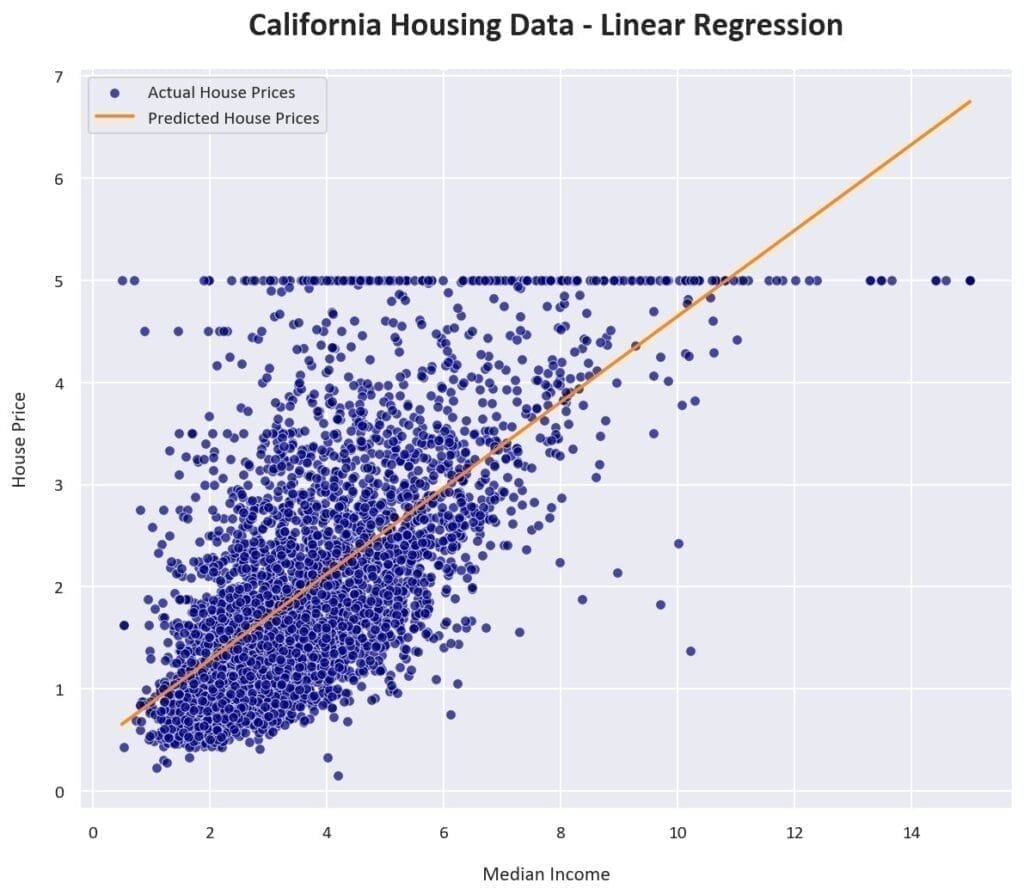
Plotting the linear regression equation on top of the data points helps us visualize how well the model fits the data. We can see that the linear regression line captures the underlying pattern in the data, but it is not a perfect fit.

This is expected, as linear regression is a simple model that assumes a linear relationship between the input and output variables. In practice, more complex models may be needed to capture the underlying patterns in the data.

Next, let’s train a multiple linear regression model using all the features in the dataset. We will use the same steps as above, but this time we will pass all the features to the model:

# Train a multiple linear regression model using all the features
X_train, X_test, y_train, y_test = train_test_split(df.drop('target', axis=1), df['target'], test_size=0.2, random_state=0)
# Create a Linear Regression model
multiple_model = LinearRegression()
# Fit the model on the training data
multiple_model.fit(X_train, y_train)
# Make predictions on the testing data
multiple_predictions = multiple_model.predict(X_test)

Next, let’s evaluate the performance of the multiple linear regression model using the same evaluation metrics as above:

As expected, the multiple linear regression model performs better than the simple linear regression model. The MAE, RMSE, are lower and the R2 score is higher, indicating that the model is better at capturing the underlying patterns in the data.

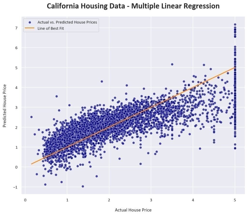
Plotting the actual vs predicted values for the multiple linear regression model shows that the model captures the underlying patterns in the data better than the simple linear regression model. The points are closer to the diagonal line, indicating that the model’s predictions are closer to the actual values.

The multiple linear regression formula determined by the model is:

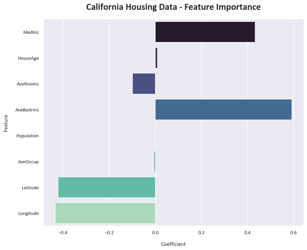
Let’s plot the feature importances of the multiple linear regression model. In this case, the feature importances are the coefficients of the linear regression model, which represent the importance of each feature in predicting the target variable.

Interestingly, the model determined that the number of bedrooms is more important than the median income in predicting house prices. This is contrary to our initial assumption that the median income would be the most important feature.

This highlights the importance of training and evaluating machine learning models to understand the underlying patterns in the data. This also means that plain correlation analysis is not enough to determine the importance of features in a predictive model.

The full source code can be found in this Github Repository.